|
Linear and Nonlinear Inverse Problems with Practical ApplicationsJennifer L. Mueller and Samuli Siltanen |
EIT with the D-bar Method: Discontinuous Heart-and-Lungs Phantom
This page contains the computational Matlab files related to the book, which you can purchase in the SIAM Bookstore.
This page is related to Example 2, a discontinuous heart-and-lungs phantom.
Introduction
The D-bar method is a reconstruction method for the nonlinear inverse conductivity problem arising from Electrical Impedance Tomography. This page contains Matlab routines implementing the D-bar method for a discontinuous heart-and-lungs phantom.
The motivation for this example comes from the following experiment:
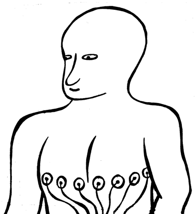
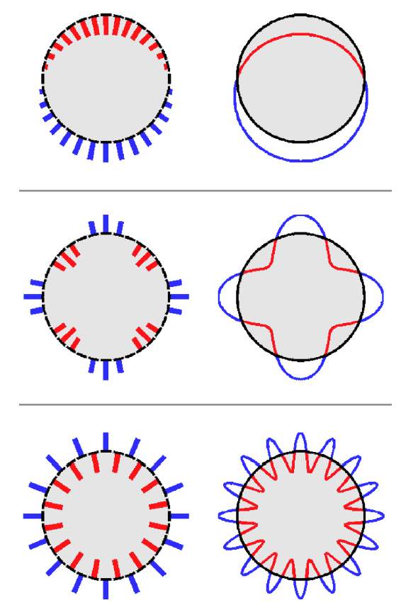
We aim to image the heart and lungs of a patient using a row of electrodes arranged as in the picture above. We think of maintaining a given voltage potential at each electrode and measuring the resulting electric current through the electrodes. This measurement is repeated for several voltage patterns. Assuming that there are 32 electrodes in total, we can use at most 31 linearly independent voltage patterns since one of the electrodes is considered as the ground potential to which the other potentials are compared to. We use trigonometric voltage patterns (examples shown below on left), approximated by continuous sine curves (below right) at the boundary:
Furthermore, we approximate the above three-dimensional (3D) situation with a two-dimensional computational model. Our virtual patient will be modelled by a two-dimensional (2D) disc with varying electrical conductivity inside. This 2D approximation, while obviously incorrect, works surprisingly well in practice.
This page is for explaining how to simulate the above kind of voltage-to-current data and how to recover the inner conductivity from the boundary measurements using the D-bar method.
Please download the Matlab routines below to your working directory and run them in the order they appear. Note that you will need the PDE Toolbox for running some of the routines.
Definition of the conductivity
Our simulated conductivity is defined in the file heartNlungs.m, and you can plot it using the routine heartNlungs_plot.m. The result should look something like this:
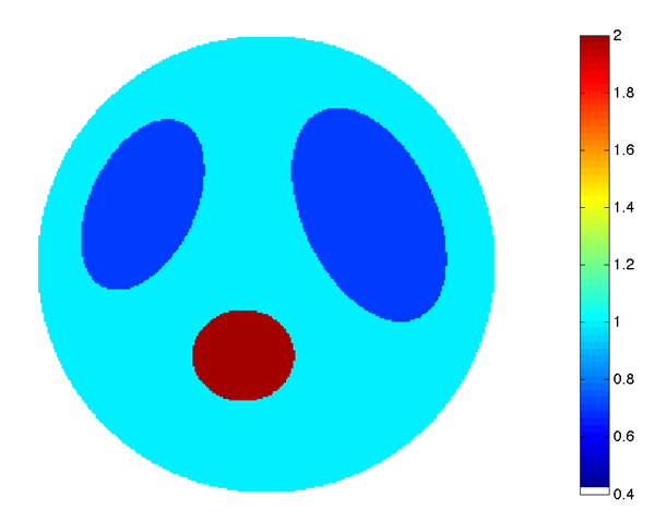
Here the background conductivity is 1, the heart is filled with blood and has higher conductivity 2, and the lungs are filled with air and have lower conductivity 0.5.
Wonder about the white color at the bottom of the colorbar above? It is for is for creating the white background in Matlab. Check out this page to learn more.
Simulation of EIT data
We simulate by first computing the current-to-voltage map using the Finite Element Method (FEM) and then inverting. In what follows, the voltage-to-current map is called DN map for Dirichlet-to-Neumann, and the current-to-voltage map is called ND map for Neumann-to-Dirichlet.
FEM is an efficient method for solving elliptic partial differential equations. The solution of the conductivity equation is given as a linear combination of basis functions that are piecewise linear in a triangular mesh. The mesh is constructed by the routine mesh_comp.m containing the parameter Nrefine. Here are plots of the triangle meshes with Nrefine=0 (left) and Nrefine=2 (right):
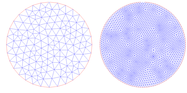
In practice it is a good idea to use Nrefine=5 for accurate results. The file mesh_comp.m saves the mesh to a file called 'data/mesh.mat'. (Note that mesh_comp.m creates a subdirectory called 'data'. If the subdirectory 'data' already exists, Matlab will show a warning. However, you don't need to care about the warning.)
The simulation of the continuum-model ND map involves solving Neumann problems of the form
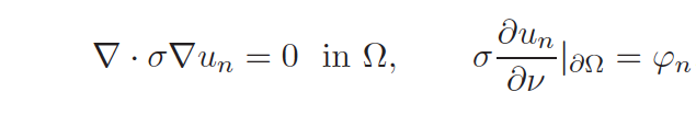
containing a Fourier basis function defined by
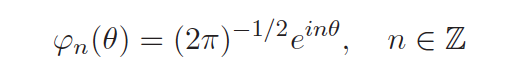
Both the Neumann condition and the conductivity given to Matlab's PDE toolbox routines as user-defined functions. Let us see how to do that. First of all, the user-defined routines need to define the functions at appropriate points related to the FEM mesh. Here are some important points:
The conductivity is constant inside each triangle, so it is naturally specified at the centers of triangles showin in (a). This is implemented in the routine FEMconductivity.m. The solution computed by FEM is represented as a function which is linear inside each triangle and thus completely determined by its values at the vertices. Therefore, the gradient of the solution is constant inside each triangle, and it is appropriate to specify the Neumann data at the midpoints (c) of boundary segments. This is done in routine BoundaryData.m. Finally, we need to find the trace of the solution for constructing the ND map; this can be done simply by picking the values of the FEM solution at the vertices (b) located at the boundary.
The routine ND_comp.m computes by FEM a matrix approximation to the ND map and saves it to data/ND.mat.
The DN map is the inverse of the ND map in the subspace of functions defined at the boundary and having mean zero. We can construct the DN matrix by first inverting the DN matrix and then adding a zero row and a zero column for dealing with the constant basis function. This is done in routine ex2DN_comp.m, which also computes the DN matrix analytically for the constant conductivity 1. The results are saved to file data/ex2DN.mat.
Computation of the scattering transform via the boundary integral equation
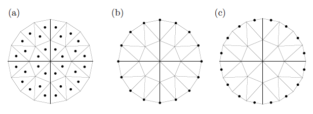
We need to construct a grid in the complex k-plane for the evaluation of the scattering transform. Download and run this file: ex2Kvec_comp.m. You can view the grid using the routine ex2Kvec_plot.m. You should see something like this:
The boundary integral equation involves a single-layer potential operator Sk with Faddeev Green's function Gk as kernel. Now Gk(z)=G0(z)+H(z,k), where G0 is the standard logarithmic Green's function for the Laplacian in dimension two and H(.,k) is a harmonic function with fixed k. We write Sk=S0+Hk, where S0 is the standard single-layer operator (known analytically for the disc domain considered here) and Hk is an integral operator with H(.,k) as kernel. We need to compute matrix approximations to the operators Hk. This is done by routine ex2Hk_comp.m, which needs the files g1.m and H1tilde.m. The matrices are saved to files data/ex2Hk_1.mat, data/ex2Hk_2.mat, ...
Note that the computation of the Hk matrices may take a long time to finish (with my MacBook pro it takes 10 hours). However, this computation needs to be done only once for a given k-grid. If the k-grid is not changed, the once-computed Hk matrices can be just loaded from the disc.
You can avoid the computation by downloading the file data.zip. Of course, if you modify ex2Kvec_comp.m to get a different k-grid, you need to actually run ex2Hk_comp.m.
Once ex2Hk_comp.m has been run (or the zip file downloaded and decompressed), we can solve the boundary integral equation for the traces of the complex geometric optics solutions. This is done by the routine ex2psi_BIE_comp.m, and the result is saved to a file in the subdirectory 'data'. The next step is to evaluate the scattering transform by integration over the boundary using the routine ex2tBIE_comp.m.
We are now ready to plot the scattering transform. Run ex2tBIE_plot.m, and you should see something like this:
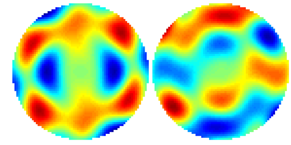
Above is shown real part (left) and imaginary part (right) of the scattering transform in the disc of radius 7.
Reconstruction from scattering transform using the D-bar method
Now we are ready to reconstruct the conductivity. Download the routines
GV_grids.m
GV_project.m
GV_prolong.m
DB_oper.m
and run ex2tBIErecon_comp.m.
You can look at the reconstruction using the routine ex2tBIErecon_plot.m. You should see something like this:
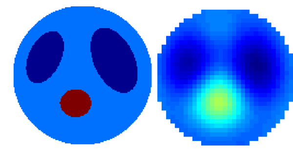
The left image shows the original conductivity distribution, and the right image shows the reconstruction using R=4. The colors (and thus numerical values) are directly comparable. Note that the reconstruction underestimates the value at the "heart."
You can try a bigger frequency cutoff radius as well. Open the file ex2tBIErecon_comp.m and change R=4 to R=6, say. You will need more accuracy, so change M = 8 into M=9 as well. The result looks like this:
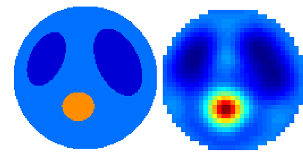
In the above picture, the colors (and thus numerical values) are directly comparable with each other. (However, the colors in the previous R=4 reconstruction image are not comparable to the R=6 image.) Note that this time the reconstruction overestimates the conductivity of the "heart;" this is a typical feature of the truncated nonlinear Fourier transform.
![]()