 |
Linear and Nonlinear Inverse Problems with Practical ApplicationsJennifer L. Mueller and Samuli Siltanen |
Matrix-free X-ray Tomography with Sparse Data
This page contains the computational Matlab files related to the book, which you can purchase in the SIAM Bookstore.
Here we solve simulated tomographic problems without constructing the measurement matrix A at all. Furthermore, we collect data with sparse angular sampling, leading to extremely ill-posed reconstruction problems.
Simulate tomographic data without inverse crime
This routine uses the radon.m function of Matlab's Image processing toolbox to create a sinogram:
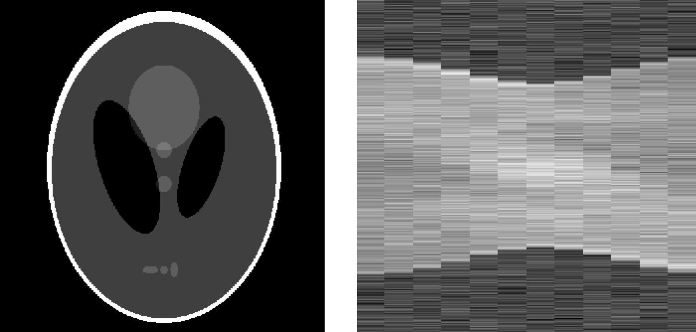
As an example we simulated data at resolution 512x512 and adding a high level of noise (10%, achieved by setting noiselevel = 0.1; in the file XRsparseA_NoCrimeData_comp.m). We use 12 parallel-beam projection directions evenly distributed over 180 degrees.
The result looks like this (original Shepp-Logan phantom on the left, sinogram on the right):
Compute reconstruction using filtered back-projection
Use this Matlab routine to compute filtered back-projection reconstructions:
As an example we simulated data at resolution 512x512 and adding a high level of noise (10%, achieved by setting noiselevel = 0.1; in the file XRsparseA_NoCrimeData_comp.m). Running the file XRsparseB_FBP_comp.m gives the following output (original Shepp-Logan phantom at left, FBP reconstruction on the right):
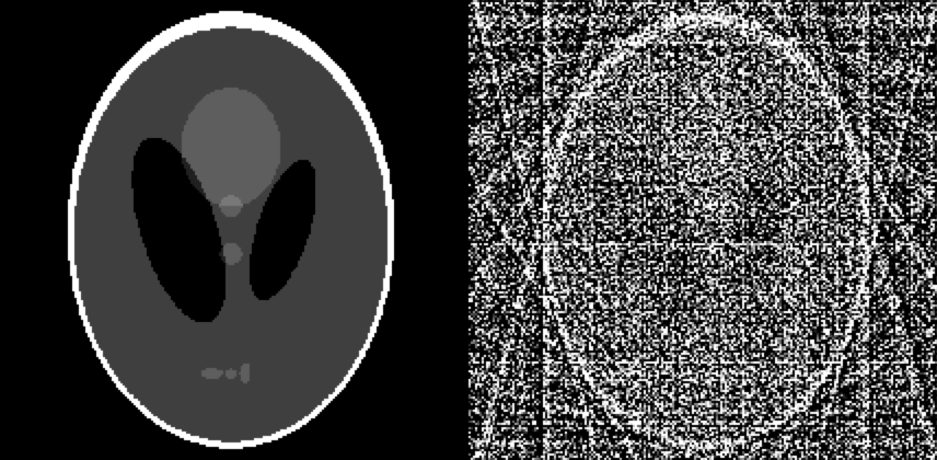
We remark that the filtered back-projection (FBP) methodology is not at all designed for sparsely sampled data considered here. FBP works very well with denser angular sampling, whenever that is available.
Also, probably FBP could be optimized to give better results even with the sparse data used here. However, that is outside the scope of this treatment.
Compute reconstruction using matrix-free iterative Tikhonov regularization
XRsparseC_Tikhonov_comp.m
XRsparseC_Tikhonov_plot.m
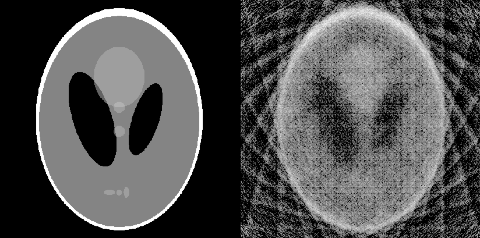
As an example we simulated data at resolution 512x512 and adding a high level of noise (10%, achieved by setting noiselevel = 0.1; in the file XRsparseA_NoCrimeData_comp.m). Then we set the following parameter values in the file called XRsparseC_Tikhonov_comp.m:
K = 600;
alpha = 300;
The result looks like this (original Shepp-Logan phantom at left, Tikhonov reconstruction on the right):
Compute reconstruction using matrix-free iterative (approximate) total variation regularization
Here are the main reconstruction and plot routines:
XRsparseD_aTV_comp.m
XRsparseD_aTV_plot.m
You will also need these files:
XR_aTV_feval.m
XR_aTV_fgrad.m
XR_aTV_grad.m
XR_aTV.m
XR_misfit_grad.m
XR_misfit.m
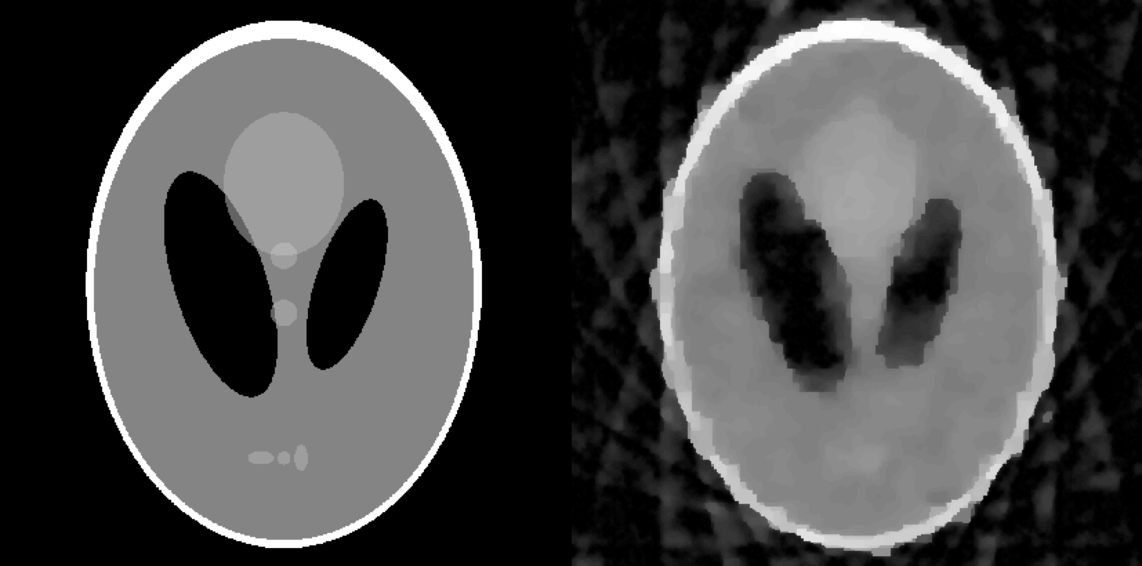
As an example we simulated data at resolution 512x512 and adding a high level of noise (10%, achieved by setting noiselevel = 0.1; in the file XRsparseA_NoCrimeData_comp.m). Then we set the following parameter values in the file called XRsparseD_aTV_comp.m:
alpha = 30000;
MAXITER = 12000;
beta = .000001;
The result looks like this (original Shepp-Logan phantom at left, approximate total variation reconstruction on the right):
![]()